Setting Up Planning Analytics AI Forecasting

In a prior issue, my colleague Brian Moore introduced us to the Forecasting feature now available in Planning Analytics Workspace (PAW). Today we take an in-depth look at the steps to set up a Preview forecast and to apply a forecast to your model.
To review, here are key steps Brian mentioned;
Drag a cube view onto the canvas and orient so that time period(s) are located on columns.
The Rows dimension should contain items in which a time series and seasonality-based prediction would provide value. Product sales by unit, net income by location, and revenue by customer are a few predictive scenarios common to most organizations.
Highlight a row for the item in which you are predicting and press the Forecast icon located on the far right of the top toolbar.
Note that several rows can be highlighted at the same time for a Forecast, and as of PAW 2.0.60 multiple rows can be previewed as well.
Be aware of the data volume when running forecasts on large consolidations as this may tie up system resources and have long calculation times.
In this article we will cover;
Preview and Forecast Defined
A Preview uses a Sandbox and does not affect your data within your TM1 model. Results are displayed in a chart. It produces statistical data to help you assess the quality of the forecast.
The Forecast operation places forecast results into the target member within your target dimension, updating your TM1 model. This operation also provides statistical details about the completed forecast.
Exploration Set-up for Forecast Preview and Forecasting
Start with an Exploration view that contains the historical periods you will base your forecast on and include the time periods that will contain your preview and forecast data.
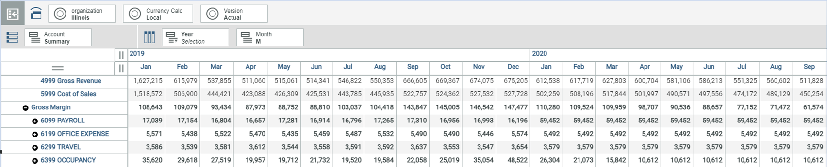
In the example above, the time dimensions define the Columns, accounts define the Rows, and Version plus Organization define the Context.
Setting Up the Time Series
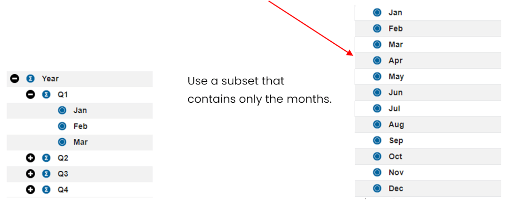
The Columns must represent a contiguous, evenly spaced time series.

In this example, two time dimensions are used, Year and Month. As they are configured, we have a continuous time series of years and months. When working with two time dimensions, make sure to arrange them so the highest level is first and your lower-level (or more finely grained) dimension is second, from left to right.

As noted above, the columns must represent an uninterrupted time series. Since the Month dimension contains some summary elements that would interfere with the forecast, a subset containing only months is used.
The forecasting function projects into all members along the time series after the chosen forecast start date. If there are any calculations or non-time members within the forecast period, then the forecast will fail.
You can also use a single time dimension that contains only years or months or weeks, etcetera. Just make sure your time series does not have any gaps and contains enough history to support your forecast.
Setting Up the Rows
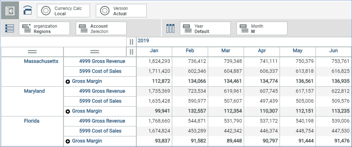
The rows of the Exploration should contain measures or metrics that change over time, like accounts (revenue, expenses) or statistics (number of products sold, returns). Rows can include nested dimensions. For example, you can combine a department dimension with expenses from the accounts dimension.
Nested Rows Example
Setting up the Context
The Context will contain the dimensions not used in the Rows or Columns. If a versions dimension is used (actual, budget, forecast), it must be included in the Context.
Important: Consolidated values are supported in the Context, but if spreading is enabled, then the Forecast function might consume a good deal of processing resources as the forecast is spread to lower levels below the consolidation. It’s advisable to test your forecast on a smaller segment of the model to ensure that you won’t have a long-running forecast process. By default, spreading by the forecast is done proportionally. You can re-spread the data using a different algorithm after forecasting.

Preview and Forecasting Options
With the Exploration oriented properly, we are ready to set the Preview and Forecast options. Click within the Exploration to highlight it and the Forecast icon will appear at the top.
Note: The preview operation runs on sandboxes and does not change your actual data.

Set Up
The Forecast panel (below) will appear on left.


Select the Forecast period start. This will be the first forecasted time period.
Select the Forecast period end. This will be the last forecasted period in the time series.
Each of the above drop-downs will contain the most granular level of your time series. In our example, it will show the year and month combined.
At the right, the forecast will start January 2022 and will end in December 2022. As a result, we will have three years of historical data to support 12 months of forecast.
Use the check box to save the statistical details as comments in the first forecasted cell.
Advanced Options
Use the Advanced features to refine your Preview and to configure your Forecast.

Auto-detect is set by default. The system will automatically detect seasonality within the historical data.

If you set Seasonality to Manual, select the number of periods seasonal changes occur. 12 is the default and might be applicable in our example, indicating a repeating yearly pattern.
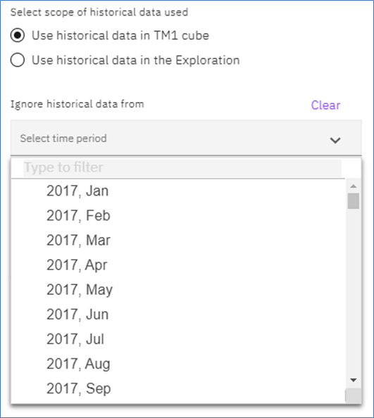
Set the scope of your historical data
Use historical data in TM1 cube uses the entire time series in the underlying cube.
Use historical data in the Exploration uses the time series in the view set in your Exploration. We recommend this option as a way to precisely control how your forecast is built. However, it may be necessary to use all data in the cube to have sufficient history.
Ignore historical data from ignores data from this point onward. If we select October 2021, then all data points after this period are ignored. This will be useful if you have incomplete data toward the end of your historical period. Use the drop-down to make your selection.

Select Confidence Interval – set the range of values that you can be reasonably certain will contain the true average of the forecasted data. In more specific terms, a 95% confidence interval means that 95% percent of the time, the true mean of the data will fall within a certain range of values.
If you want to save the Forecast results (by clicking the Forecast button), update the following, else, for Preview only, you can leave these fields blank.

For this example, we created special versions within the Version dimension to house the forecasted data, and the upper and lower bounds.
Where do you want to save the predicted values?
Select dimension - You can save the forecast results to a member within a specified dimension. We have a Forecast AI version set up in the Version dimension that was created for this purpose. However, it could go into any dimension open for data entry and it must be in the Context.
Select the hierarchy – if there are no hierarchies, the default hierarchy will have the same name as the dimension.
Select member to save prediction – enter the version to house your forecast.
Select member to save upper bound (optional) – select the dimension member where the upper range of the confidence interval will be saved.
Select member to save lower bound (optional) – select the dimension member where the lower range of the confidence interval will be saved.
Click the Save upper and lower bound for consolidations check box to save upper and lower bound consolidations.
After a selection is made from the drop-downs, an X appears to the left of the drop-down arrow. Click on the X to remove\clear the selection.
With the set-up complete we can proceed to the Preview and Forecast operations.
Preview Example
Select up to 25 rows. If more than 25 rows are selected, the Preview button is disabled. In the following example, one row is selected and Preview is enabled.
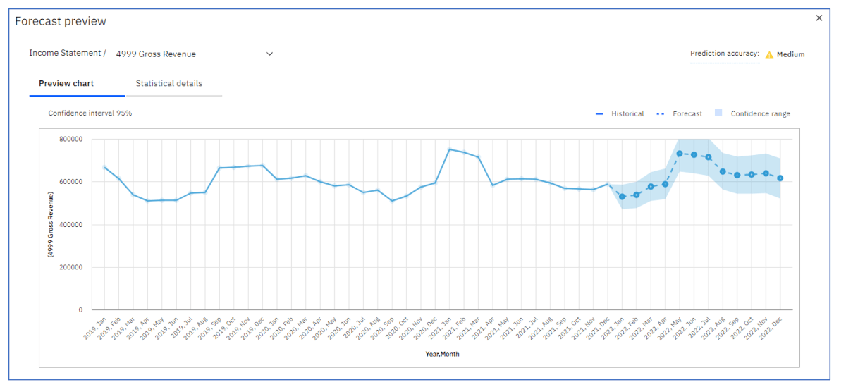
Starting with the Exploration view below, 4999 Gross Revenue is highlighted and the Set-up is complete, click Preview.

In a few seconds the Forecast Preview chart appears.
Note the Prediction accuracy and Confidence range.
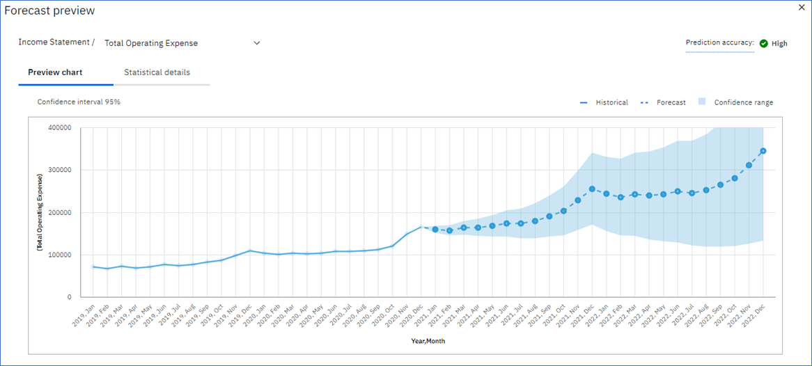
Using another account, Total Operating Expense, we get a high Prediction accuracy. We see a discernible trend and some seasonality.

Click on or hover over Prediction accuracy to see the meaning of High, Medium, and Low.

Prediction accuracy is an important indicator of the usefulness of a prediction and represents how well the model was able to fit the historical data. If the accuracy is low, then the exponential smoothing model that was used was not a good fit for this data. The prediction is likely not usable.
If you choose more than one row to preview, you can see each row by clicking the drop-down arrow to the left of the row name.


Forecast Preview Statistical
We cover the specifics of the Statistical details later in this article. Click the Learn more link for explanations of each statistic.

Forecasting Example
Start the Forecast process from an Exploration.
In our example, we are using the same Exploration configuration and Advanced Options selected earlier.

Like Preview, Forecasting requires the time dimension(s) to form the columns. Also, like the Preview, the time dimension must be a contiguous, evenly spaced time series.
Unlike Preview, Forecast will not produce a chart. You can create a chart after the forecast operation is complete. See the example chart under the Forecast Results section.
Highlight the rows you want to forecast and click the Forecast button.
Based on the selections, the system will place the resulting forecast in the target version along with amounts for the upper and lower bounds of the confidence interval (if designated).

After the Forecast is complete, the Forecast set-up panel will contain a Result summary including when the forecast was last launched.
Click on the Details link to see the detail on additional time series used in the Forecast. If you used only one time series, the details will appear again here.
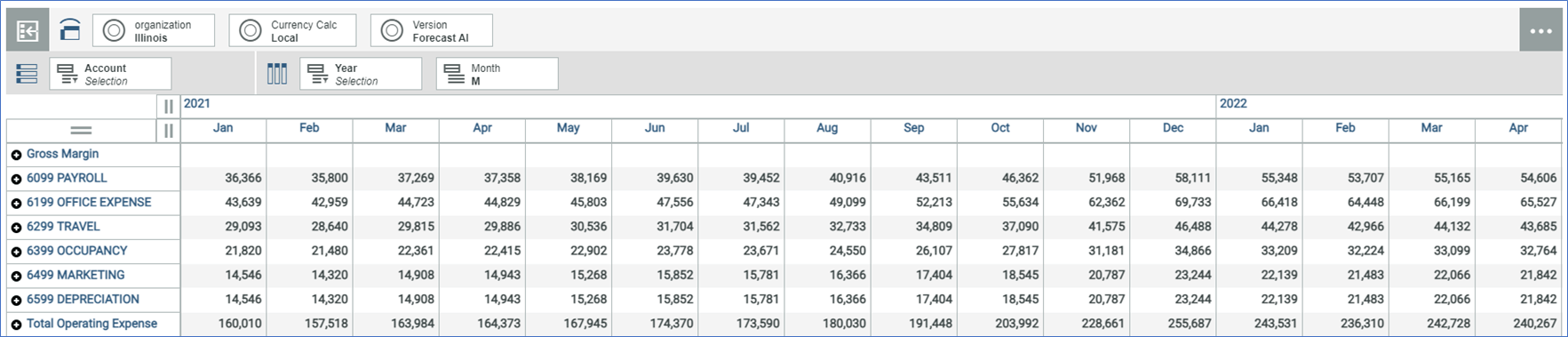
Forecasted Amounts
Note that the components of Total Operating Expense are also populated. Total Operating Expense was selected, and the Forecast process spread the forecasted values to the accounts that sum to Total Operating Expense.
Forecasted Total Operating Expenses with Upper Bound and Lower Bounds
Based on our selections within the Advanced Options, our example forecast went to the Forecast AI member within the Version dimension with the upper and lower bounds going to the Forecast AI Upper and Forecast AI Lower members respectively.

Chart for Forecast AI with Upper and Lower Bounds

About the Forecast Calculations
Preview and Forecast use one of nine exponential smoothing models*. The type of model the system chooses is dependent on the historical data and whether trends or seasonality is detected. The system iterates through the historical data to detect trends and seasonality and then builds predictions. The model with the predictions that best fit the historical data is used.
Using the Total Operating Expense example, we have the Preview chart and Statistical details.

Accuracy Details
The Accuracy Details provide information on how well the chosen model matched the historical data. All accuracy measures are based on the historical data.
AIC (Akaike Information Criterion)
A model selection measure. It compares the quality of a set of statistical models to each other. The AIC will take each model and rank them from best to worst. The best model will be the one that neither under-fits nor over-fits the historical data. The model with the lowest AIC is deemed the best model. The AIC shown in Accuracy Details is the AIC of the chosen model.
MAE (Mean Absolute Error)
Measures the average magnitude of the errors between the values fitted by the model and the observed historical data. It’s the average over the test sample of the absolute differences between prediction and actual observation where all individual differences have equal weight.
MAPE (Mean Absolute Percent Error)
The average absolute percent difference between the values that are fitted by the model and the observed data values.
MASE (Mean Absolute Scaled Error)
The error measure that is used for model accuracy. It is the MAE divided by the MAE of the naive model. The naive model predicts the current period’s value as the previous period’s actual value. Scaling by this error means that you can evaluate how good the model is compared to the naive model. If the MASE is greater than 1, then the model is worse than the naive model. The lower the MASE, the better the model is compared to the naive model.
Accuracy (Accuracy %)
The primary indicator of the model accuracy based on the fitted values. It is specified as the reduction percentage of mean absolute error relative to the naïve model. It is computed by subtracting MASE from 1 and expressing it as percentage. If MASE is greater than or equal to 1, the accuracy is set to 0% because the model does not improve upon the naïve model. Higher accuracy indicates lower model error relative to the naïve model.
MSE (Mean Squared Error)
The mean squared error tells you the difference between values fitted by the model and the historical values. MSE is calculated by taking the sum of squared differences between the values that are fitted by the model and historical values, divided by the number of historical points, minus the number of parameters in the model. It is the average of the set of calculated errors. The lower the number, the better.
RMSE (Root Mean Squared Error)
The square root of the MSE. RMSE is a measure (standard deviation) of how spread out the “errors” are. In other words, it tells you how concentrated the historical data is around the line of best fit.
Parameters
Detected Seasonal period and estimates for other parameters that are used in the selected exponential smoothing model are available.
Alpha (Base Factor)
The smoothing factor for level states in the exponential smoothing model. Small values of alpha increase the amount of smoothing, that is, more history is considered when the alpha is small. Large values of alpha reduce the amount of smoothing, which means that more weight is placed on the more recent observations. When the alpha is 1, all the weight is placed on the current observation.
Beta (Trend Factor)
The smoothing factor for trend states in the exponential smoothing model. This parameter behaves similar to alpha, but is for trend instead of level states. Beta determines the degree to which recent data trends should be valued compared to older trends when making the forecast. The higher the Beta, more weight is given to more recent trends and a lower Beta emphasizes older trends. Beta value is restricted between 0 and 1.
Gamma (Seasonal Factor)
The smoothing factor for seasonality states in the exponential smoothing model. Serves the similar role as alpha, but for the seasonal component of the model. The seasonal component is the repeating pattern of the forecast. The higher the Gamma, the more recent seasonal pattern is emphasized. Gamma is restricted between 0 and 1.
More Information
For more information on statistical details and other forecast features, see the Planning Analytics Workspace documentation.
*Exponential smoothing models are applicable to a single set of values that are recorded over equal time increments only. They support data properties that are frequently found in business applications such as trend, seasonality, and time dependence. All specified model features are estimated based on available historical data. An estimated smoothing model can then be used to forecast future values and provide upper and lower confidence bounds for the forecast values. Each model type is suited for modeling a different combination of properties that are found in the data like trend and seasonality. The exponential smoothing model chosen by Planning Analytics is based on the model that best matches the historical data.
Next Steps
We hope you found this article informative. Be sure to subscribe to our newsletter for data and analytics news, updates, and insights delivered directly to your inbox.
If you have any questions or would like PMsquare to provide guidance and support for your analytics solution, contact us today.
